Define an algorithm and explain why algorithms — not computers — are the central idea in computer science
Read pseudocode and a simple flowchart, and translate between pseudocode and Python
Trace a small Python program line by line and predict its output
Describe how computing hardware evolved from mechanical gears (1840s) to integrated circuits (1960s) and what each generation made newly possible
Use an AI assistant to draft or modify code, and verify the result before trusting it
What Is Computer Science?
A common first guess: computer science is about computers. That’s close — but it’s a bit like saying astronomy is about telescopes. The telescope is the tool; the stars are the subject.
Computer science is the study of algorithms — step-by-step procedures for solving problems. Computers are the machines we use to run algorithms quickly, but the algorithms themselves are older than any electronic computer. Some of the most important ones were invented on paper, by hand, long before a machine existed to execute them.
The field has several major branches:
Theory — what problems can be solved by a machine? How efficiently?
Systems — how do we build hardware and software that runs algorithms reliably?
Data — how do we store, retrieve, and make sense of information?
Intelligence — can we write algorithms that learn from experience?
Security — how do we protect systems and the people who depend on them?
In this notebook, we’ll meet four landmark algorithms, trace how they worked, and see what kind of machine each one ran on. That machine matters: the hardware of each era shaped what algorithms were even imaginable.
The Four Algorithms We’ll Study
#
Algorithm
Year
What it did
1
Lovelace’s Note G
1843
Computed a mathematical sequence on a proposed mechanical engine
2
Hollerith’s Tabulator
1890
Counted and grouped millions of census records
3
Turing’s Bombe
1940s
Broke Nazi military encryption
4
Weizenbaum’s ELIZA
1966
Held a typed conversation by pattern-matching
Each one solved a real, urgent problem. Each one also pushed the boundaries of what contemporary hardware could do — often before the hardware was even finished being built.
A Hundred and Twenty Years of Hardware
The four algorithms didn’t run on laptops. They ran on fundamentally different machines, and the hardware shaped what was possible.
Era
Switching element
How it stored data
Rough speed
1840s
Mechanical gears (steam-powered)
Positions of brass wheels
~1 addition / second (designed)
1890s
Electromechanical relays
Punch cards + mechanical counters
~1 card / second
1940s
Vacuum tubes + rotors
Paper tape, plugboards
~5,000 operations / second
1960s
Transistors, integrated circuits
Magnetic core + tape
~300,000 operations / second
Each generation was roughly 1,000× faster than the last. A 2026 smartphone runs billions of operations per second — another ~10,000× jump beyond the 1960s. Yet the basic ideas — loops, conditions, lookup tables, pattern matching — have barely changed since Lovelace wrote them down.
Getting Set Up: Google Colab
This course runs in Google Colab — a free, browser-based Python environment. No installation required. You need a Google account.
A Colab notebook is made of cells: - Text cells — formatted prose like this one (Markdown format) - Code cells — Python you can run with Shift + Enter or the ▶ button
To save your work:File → Save a copy in Drive. Colab also auto-saves as you go.
Run the code cell below.
# The # symbol starts a comment. Python ignores comments — they're for human readers.print("Hello. I am a computer. I follow instructions.")print("I do not understand what those instructions mean.")print("That distinction will matter a great deal this semester.")
Hello. I am a computer. I follow instructions.
I do not understand what those instructions mean.
That distinction will matter a great deal this semester.
What just happened, line by line:
print(...) is a built-in function — code that comes with Python. It displays whatever you put inside the parentheses.
The text in quotes is a string — a sequence of characters.
Python executed the three lines in order, top to bottom. That sequential execution is the most fundamental property of an algorithm: the steps happen in a defined order.
Your AI Pair-Programmer
Colab has a built-in AI assistant (Gemini — the ✨ icon or the button in the top-right corner). You can also use Claude (claude.ai) or ChatGPT (chat.openai.com) in a separate tab.
The single most important rule:
AI is a fast first draft, not a final answer. Your job is to verify.
You verify by: - Running the code and checking the output - Testing it on inputs where you already know the right answer - Reading it carefully enough to spot something suspicious - Asking yourself: does this do what I asked, or just something that sounds like it?
Every notebook in this course will include AI-assisted exercises. You’ll get fast at this.
# Open Gemini (or Claude / ChatGPT) and send this prompt:## "Write a Python function that takes a name as input and returns# a greeting string. Include a type hint and a one-line docstring."## Paste the result below this line, run it, and check the output.
Algorithm 1 — Lovelace’s Sequence (1843)
The Problem
Nineteenth-century science needed long, accurate tables of numbers — logarithms, ship navigation tables, insurance calculations. These tables were computed by hand, by rooms of human “computers” (that was a job title, not a machine). Humans made mistakes. Mistakes in a navigation table could wreck a ship.
Charles Babbage proposed to fix this with a mechanical calculator. His second design, the Analytical Engine, was far more ambitious than the first: it would be general-purpose — not a single-task calculator but a machine that could follow any sequence of instructions fed to it.
Ada Lovelace, a mathematician and Babbage’s correspondent, wrote a set of notes describing what the engine could do. In her longest note — Note G — she included a detailed procedure for computing a mathematical sequence called the Bernoulli numbers. This is widely regarded as the world’s first computer program, though authorship was collaborative — Babbage drafted earlier procedures, while the Bernoulli table and the broader claims about what the machine could do were Lovelace’s own.
The Hardware: Babbage’s Analytical Engine
The Analytical Engine was never completed — it was too complex to build with Victorian manufacturing. But Babbage’s design describes a machine shockingly close to a modern computer.
Modern name
Babbage’s name
What it did
CPU
The Mill
Performed arithmetic on numbers
RAM
The Store
Held 1,000 numbers of 40 digits each
Program input
Operation cards
Punched cards telling the Mill what to do
Data input
Variable cards
Punched cards telling it which numbers to use
Output
Printer + card punch
Printed results; punched cards for reuse
Physical reality: - Would have been the size of a small locomotive - Powered by a steam engine turning brass gears - Expected speed: roughly one addition per second (a multiplication took about a minute) - The punch-card idea came from the Jacquard loom, a French weaving machine that used cards to select thread patterns
Lovelace’s program was written on paper for a machine that did not yet exist — and would not exist in her lifetime.
Picture It: the Analytical Engine
Babbage’s design maps cleanly onto a modern computer. The diagram below shows the four parts from the table above and how data and instructions flow between them.
Reading it: the Mill is the CPU and the Store is memory; operation cards bring the program, variable cards bring the data, and results flow back out — the von Neumann shape, a century early.
The Algorithm in Pseudocode
Bernoulli numbers are complicated. For our purposes, we’ll use a simpler sequence that captures the same structure: the factorials (1! = 1, 2! = 2, 3! = 6, 4! = 24, …). Factorials have the same kind of structure as Bernoulli: each term builds on the previous one.
Before we write Python, we write pseudocode — plain-English steps, structured clearly enough that any programmer could translate them into any language.
ALGORITHM: compute_factorials
INPUT:     n — a positive integer
OUTPUT:    a list of the first n factorials: [1!, 2!, ..., n!]

1. CREATE an empty list called results
2. SET running_product = 1
3. FOR each number i from 1 to n:
       3a. MULTIPLY running_product by i
       3b. APPEND running_product to results
4. RETURN results
Notice what pseudocode is not: it isn’t Python. There are no colons, no parentheses, no particular syntax. It’s a way of thinking clearly about the steps before committing to a language.
Reading it: the diamond is the loop test; the back-arrow is the repetition; running_product is multiplied each pass. The Python next is a line-for-line translation of this.
# The same algorithm in Python.def compute_factorials(n):"""Return a list of factorials from 1! to n!.""" results = [] running_product =1for i inrange(1, n +1): running_product = running_product * i results.append(running_product)return resultsprint(compute_factorials(6))
[1, 2, 6, 24, 120, 720]
Walking Through the Code
def compute_factorials(n): — defines a function named compute_factorials that takes one input, n. A function is a named, reusable block of code.
results = [] — creates an empty list. Lists hold sequences of values. This is where we’ll collect the factorials as we compute them.
running_product = 1 — our accumulator: a variable that carries a value from one loop step to the next. It starts at 1 because multiplying anything by 1 leaves it unchanged.
for i in range(1, n + 1): — a loop. range(1, n + 1) generates the numbers 1, 2, 3, …, n. (The + 1 is because rangestops before the second number, so range(1, 7) gives 1–6.)
running_product = running_product * i — update the accumulator. On the third pass, this computes 1 × 1 × 2 × 3 = 6 = 3!.
results.append(running_product) — add the current value to the end of the list.
return results — when the loop is done, hand the list back to whoever called the function.
Two core patterns to watch for all semester: - Accumulator — a variable that builds up a result across loop iterations - Function — a named, reusable block of instructions (Lovelace’s subroutine)
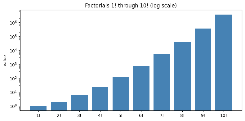
Picture It: How Fast Factorials Grow
Numbers from a loop can balloon fast. The chart below plots 1! through 10! on a log scale so the explosive growth is visible.
10! = 3,628,800
The values grow explosively — 10! is already over three million. That’s the accumulator compounding at every step. Small algorithms can produce enormous outputs; this will be true throughout the course.
Cultural note. Twenty-five years before Note G, Lovelace’s friend Mary Shelley published Frankenstein — a novel about what happens when a maker brings something into the world and can’t control what it does next. Lovelace was quietly designing the mathematical version of the same question: a machine that follows instructions without a human deciding each step. We’ll return to that question throughout the semester.
✏️ Exercise 1 — Lovelace’s Table 🤖 AI-Assisted
Open Gemini (or Claude / ChatGPT) and send it this prompt:
“I have a Python function compute_factorials(n) that returns a list of factorials from 1! to n!. Extend it to print a formatted table with three columns: n, n!, and the ratio n! / (n − 1)!. Use f-strings for column alignment.”
Then: 1. Paste the AI-generated function into a new code cell and run it for n = 8. 2. Find one thing you’d improve — formatting, variable names, an edge case. 3. Fix it and re-run. 4. In a markdown cell, write 2–3 sentences: what did you change, and why?
Algorithms for Mathematics from Lovelace to the Present
Ada Lovelace’s Note G envisioned a machine that could weave algebraic patterns just as the Jacquard loom wove flowers and leaves. Her focus on computing the Bernoulli numbers was just the beginning. Over the next century and a half, the evolution of computing hardware allowed mathematicians to solve increasingly complex problems, proving that algorithms are as essential to modern mathematics as the telescope is to astronomy.
Here are five major milestones where computers were used to push the boundaries of mathematics:
Artillery Trajectories (1940s): The ENIAC, one of the first electronic general-purpose computers, was initially designed to calculate complex differential equations for artillery firing tables during WWII.
Monte Carlo Methods (1940s): Stanislaw Ulam and John von Neumann developed randomized algorithms to simulate neutron diffusion, birthing computational probability and modern simulation.
The Fast Fourier Transform (1965): An algorithm popularized by Cooley and Tukey that dramatically reduced the time needed to compute the discrete Fourier transform, revolutionizing digital signal processing and applied mathematics.
The Four Color Theorem (1976): The first major mathematical theorem proved using a computer. The program checked 1,936 distinct configurations to show that any map can be colored with just four colors without adjacent regions sharing a color.
AI-Assisted Theorem Proving (2020s): Today, systems like Lean (a formal proof assistant) and AI models are being used not just to verify human proofs, but to help discover new mathematical insights, theorems, and bounds in fields like combinatorics and geometry.
💭 Think About It — Can You Trust a Proof You Can’t Read?
The Four Color Theorem (1976) was the first famous result whose proof no human could fully check by hand — a computer had to grind through nearly two thousand cases. Today, AI systems help discover proofs as well as verify them.
If a theorem is “proved” only because a machine checked more cases than any person could read in a lifetime, do you count it as proved? What would it take to convince you?
Lovelace insisted her machine “has no pretensions to originate anything” — it only does what we order it to. Does AI-assisted mathematics challenge that claim, or is it still just following orders very fast?
Think of a time you trusted an answer from a calculator, a spreadsheet, or an app without checking it yourself. What made you trust it? Was that trust earned?
There are no single right answers here — share a sentence or two on each.
Algorithm 2 — Hollerith’s Tabulator (1890)
The Problem
The US Constitution requires a census every ten years. The 1880 census took eight years to process by hand — nearly obsolete by the time it was published. If the 1890 census took any longer, the results wouldn’t be ready before 1900.
Herman Hollerith, a young statistician who had worked on the 1880 count, proposed a radical solution:
Record each person’s answers as holes punched in a card — one card per person
Feed cards into a machine that senses the holes electrically
Let the machine count and sort faster than any human
The 1890 census was complete in one year. Hollerith’s company eventually became IBM.
The Hardware: Punch Cards and Electromechanical Relays
Hollerith’s system had three parts:
The card. A piece of stiff paper about the size of a dollar bill. Specific hole positions represented specific answers (age ranges, occupation categories, state of birth, and so on). A card was essentially a fixed-width record — the same concept used by every modern database.
The tabulator. An operator placed a card in a press. Metal pins dropped toward the card. Where there was a hole, a pin passed through and dipped into a cup of mercury below, completing an electrical circuit. Each circuit advanced a mechanical counter for that category.
The sorter. A separate machine used the same electrical sensing to drop cards into different physical bins based on any chosen hole position — allowing the operator to regroup the data and count it again by some other criterion.
Why this was a huge leap:
Human clerks
Hollerith’s machines
Medium
Paper tally sheets
Punch cards
Error rate
Tired clerks miscount
Electrical pins are consistent
Re-grouping data
Re-sort all paper
Re-run cards through the sorter
Speed
Days to months
Hours
Hollerith’s machines couldn’t run arbitrary programs — they were hardwired for counting and sorting. But the data format (a record with fixed fields) is the direct ancestor of the dictionaries and database rows you’ll use for the rest of your career.
The Algorithm in Pseudocode
We’re going to replicate Hollerith’s core operation: group records by a category, count each group.
ALGORITHM: count_by_field
INPUT:     records — a list of records (each with the same fields)
           field   — the name of the field to group by
OUTPUT:    a dictionary mapping each value of that field to its count

1. CREATE an empty dictionary called tally
2. FOR each record in records:
       2a. LOOK UP the record's value for the given field → call it key
       2b. IF key is already in tally:
              ADD 1 to tally[key]
           OTHERWISE:
              SET tally[key] = 1
3. RETURN tally
Notice: the mechanical version (Hollerith) used pins, circuits, and counters. The Python version uses a dictionary. The logic is identical.
# Each person is a Python dictionary (like one of Hollerith's cards).# The whole list is our "stack of cards."census_records = [ {"name": "Mary Shelley", "state": "NY", "occupation": "writer"}, {"name": "Ada Lovelace", "state": "MA", "occupation": "mathematician"}, {"name": "Herman Hollerith","state": "NY", "occupation": "engineer"}, {"name": "Frederick Law", "state": "MA", "occupation": "farmer"}, {"name": "Clara Barton", "state": "NY", "occupation": "nurse"}, {"name": "Thomas Edison", "state": "NJ", "occupation": "engineer"}, {"name": "Ida B. Wells", "state": "IL", "occupation": "journalist"}, {"name": "George Pullman", "state": "IL", "occupation": "industrialist"},]def count_by_field(records, field):"""Group records by `field` and return counts.""" tally = {}for record in records: key = record[field]if key in tally: tally[key] = tally[key] +1else: tally[key] =1return tallyprint(count_by_field(census_records, "state"))print(count_by_field(census_records, "occupation"))
census_records = [...] — a list of dictionaries. Each {...} is one person; each person has three labeled fields.
def count_by_field(records, field): — this function takes two inputs: the list of records, and the name of the field to group by (a string like "state").
tally = {} — an empty dictionary. Dictionaries store values by named keys, not by position.
for record in records: — loop through the records one at a time. Each pass, record is one person’s dictionary.
key = record[field] — look up that person’s value for the field. If field is "state" and the record is Ada Lovelace’s, key becomes "MA".
if key in tally: — have we seen this category before?
Yes:tally[key] = tally[key] + 1 — increment the existing count.
No:tally[key] = 1 — create a new entry starting at 1.
return tally — once every record has been processed, return the finished dictionary.
Two new Python ideas here: - Dictionary — a lookup table: keys map to values ({"NY": 3, "MA": 2}). Dictionaries are everywhere: JSON, database records, config files, function arguments. - List of dictionaries — a mini database table. One of the most useful structures you’ll meet this semester.
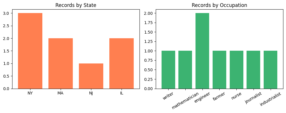
Picture It: the Tally, Charted
The same count_by_field function answers two different questions. The bars below show its output grouped by state and by occupation, side by side.
The same function answered two different questions about the same data. Hollerith’s machines worked the same way — you changed which hole positions they read, and the same hardware counted something different. Writing a general function (not a count_by_stateand a count_by_occupation) is called abstraction, and it’s one of the most powerful ideas in programming.
Cultural note. In 1872, Samuel Butler’s novel Erewhon imagined a civilization that had banned its machines out of fear they were slowly evolving toward consciousness. When Hollerith’s tabulator replaced a room of clerks eighteen years later, Butler’s readers could be forgiven for feeling vindicated. The machines weren’t smarter — just faster. This time, at counting people.
✏️ Exercise 2 — Hollerith’s Census, Your Way
No new code to write here. You’ll use the count_by_field function from above and watch how its answers change as you poke at it.
Ask a different question. In a new code cell, run count_by_field(census_records, "occupation") and print the result. How is this answer different from grouping by "state"?
Add yourself to the census. In the census_records cell, copy one of the {...} record lines and change the name, state, and occupation to your own (invent any state you like). Re-run that cell, then re-run your call from step 1. Which count went up by one?
Predict, then check.Before running, write a one-line prediction in a markdown cell: if you change your record’s state to "NY", what will the "NY" count become? Then run it and see whether you were right.
That’s the whole point of this function: one small piece of code answers many questions, on data that keeps changing. Reusing one tool across many cases like this is called abstraction — an idea you’ll meet again and again.
Computers for Data Analysis from Hollerith to the Present
Herman Hollerith’s punch card tabulator revolutionized data processing by drastically reducing the time needed to tabulate the 1890 census. This foundational idea of representing data as structured, machine-readable records paved the way for the modern data ecosystem. Over the next century, breakthroughs in hardware storage and software abstraction transformed how we collect, store, and analyze information.
Here are five major milestones in the evolution of computers for data analysis:
Magnetic Storage (1950s): The invention of magnetic tape and the first hard disk drives (like the IBM RAMAC) replaced bulky punch cards, allowing for vastly greater storage density and faster, random access to records.
Relational Databases (1970s): Edgar F. Codd invented the relational database model at IBM. This shifted data storage from rigid, physical hierarchies into flexible tables linked by common fields, laying the groundwork for SQL and modern data management.
The Electronic Spreadsheet (1979): The release of VisiCalc (and later Excel) brought intuitive, interactive data analysis to personal computers, allowing users to instantly recalculate entire sheets when a single variable changed.
Distributed Computing & Big Data (2000s): As internet traffic and data collection exploded, distributed file systems and processing frameworks (like Hadoop and MapReduce) were created to store and analyze petabytes of unstructured data across thousands of commodity servers.
Cloud Data and DataFrames (2010s–Present): The rise of cloud data warehouses (like Snowflake or BigQuery) combined with powerful, open-source software abstractions (like Python’s pandas library) democratized data science, enabling analysts to process massive datasets with just a few lines of code.
💭 Think About It — Counting People
Hollerith’s tabulator was built to count a whole nation. The moment you turn people into rows of data, you can answer questions about them at astonishing speed — and that power cuts both ways.
What genuinely good things become possible when a government or company can quickly count and sort millions of people (think public health, services, planning)?
A category recorded for one harmless reason can later be used for a purpose no one intended when the data was collected. Why might that be hard to prevent, even with good intentions at the start?
You are a “row” in dozens of databases right now. Describe one way you’ve noticed being treated as a data point. Did it feel helpful, unsettling, or both?
There are no single right answers here — share a sentence or two on each.
Algorithm 3 — Turing’s Codebreaker (1940s)
The Problem
During World War II, Nazi Germany encrypted its military communications with a device called Enigma. Each day, operators set their machines to a new configuration — a key — before transmitting. Without the key, messages looked like random letters. With the key, they decoded instantly.
The search space was astronomical: - Enigma had ~158 million million million (1.58 × 10²⁰) possible settings - That’s more settings than grains of sand on all the beaches on Earth - Testing them one at a time, even at one per second, would take longer than the age of the universe
Alan Turing’s key insight: don’t try every setting — eliminate the wrong ones fast. German messages had predictable content (weather reports started with weather words; routine messages ended with stock phrases). If you knew what a few plaintext words should look like, you could rule out most settings almost immediately.
The Hardware: Enigma, the Bombe, and Colossus
Three machines sat at the heart of this story:
1. The Enigma machine (Germany, 1920s–1940s). A typewriter-sized device with three rotating wheels (rotors), a plugboard of swappable wires, and a reflector. Pressing a key sent electricity through the rotors and plugboard; a lamp lit up the encrypted letter. After each keystroke, the rotors advanced — so the same letter typed twice produced two different ciphertexts.
2. The Bombe (Bletchley Park, 1940). Turing’s codebreaking device. Not a general computer — a special-purpose electromechanical machine built to test Enigma configurations rapidly. Roughly 6 feet tall, 7 feet wide, filled with rotating drums that simulated Enigma wheels. It could check thousands of settings per minute.
3. Colossus (Bletchley Park, 1943). Used against a different German cipher, not Enigma. But worth knowing: Colossus was the world’s first programmable electronic digital computer. It used about 1,500 vacuum tubes — fragile glass bulbs acting as electronic switches. Vacuum tubes were 1,000× faster than the mechanical relays of Hollerith’s era.
The hardware shift that mattered: mechanical parts (moving) → electromechanical relays (switching magnetically) → vacuum tubes (switching electronically, with no moving parts). Each step made computing faster and made algorithms that used to take weeks feasible in hours.
The Algorithm in Pseudocode
Enigma is complicated. We’ll study the Caesar cipher — a much simpler cipher that shares Enigma’s core idea: shift each letter by some amount. Break the Caesar cipher, and you understand the shape of the problem Turing was solving at scale.
ALGORITHM: caesar_encrypt
INPUT:     plaintext — a string of letters and other characters
           shift     — an integer between 0 and 25
OUTPUT:    the encrypted string

1. SET result = empty string
2. FOR each character c in plaintext:
       2a. IF c is a letter:
              shift c by `shift` positions in the alphabet
              wrap around from Z back to A
              APPEND the new letter to result
           OTHERWISE:
              APPEND c to result unchanged
3. RETURN result
def caesar_encrypt(plaintext, shift):"""Encrypt a string by shifting each letter by `shift` positions.""" result =""for c in plaintext.upper():if c.isalpha(): shifted = (ord(c) -ord('A') + shift) %26 result = result +chr(shifted +ord('A'))else: result = result + creturn resultmessage ="THE EAGLE HAS LANDED"encrypted = caesar_encrypt(message, 13)print(f"Original: {message}")print(f"Encrypted: {encrypted}")
Original:  THE EAGLE HAS LANDED
Encrypted: GUR RNTYR UNF YNAQRQ
Walking Through the Code
Three new Python tools appear here:
ord(c) — returns the numeric code of a character. ord('A') is 65, ord('B') is 66, ord('Z') is 90.
chr(n) — the reverse: chr(65) is 'A'.
% — the modulo operator, which returns the remainder after division. 27 % 26 = 1, 52 % 26 = 0. This is what wraps letters around: if you shift Z by 1, you get A, not some off-the-end character.
Line by line: - for c in plaintext.upper(): — loop through each character of the uppercased input. - if c.isalpha(): — only shift letters; leave spaces and punctuation alone. - shifted = (ord(c) - ord('A') + shift) % 26 — this is four operations: 1. ord(c) - ord('A') — convert the letter to a 0-based index (A=0, B=1, …, Z=25) 2. + shift — move it forward by shift positions 3. % 26 — wrap around if we went past Z 4. (The result is still a number 0–25) - chr(shifted + ord('A')) — convert back to a letter (add 65 to get back into ASCII, then chr gives us the character).
# Turing's move, in miniature: try every possible shift, and let a human# spot the one that reads like English.def caesar_brute_force(ciphertext):"""Print all 25 possible decryptions."""print(f"Ciphertext: {ciphertext}\n")for shift inrange(1, 26): attempt = caesar_encrypt(ciphertext, 26- shift)print(f"Shift {shift:2d}: {attempt}")caesar_brute_force(encrypted)
Scan the output. Exactly one line reads like English. A human spots it immediately; a simple dictionary-check program could spot it automatically. That’s the shape of codebreaking:
Generate every possible answer systematically
Filter out the ones that are obviously wrong
Let a human (or a simple checker) recognize the right one
Turing’s Bombe did a more sophisticated version of the same three steps — at thousands of configurations per minute. Historians estimate this work shortened the war in Europe by two to four years and saved millions of lives. Turing received no public recognition during his lifetime; he was prosecuted in 1952 for being gay and died in 1954 at age forty-one.
Cultural note. In the same year Colossus was dismantled on Churchill’s orders, George Orwell finished Nineteen Eighty-Four — a novel about a state that watches every communication. The math Turing used to defeat a surveillance regime is the same math a surveillance regime would use against its own citizens. Both uses are still with us.
✏️ Exercise 3 — Driving the Caesar Cipher
No code to write here. You’ll call the caesar_encrypt function over and over with different inputs and watch what comes back. Feeding a function things and reading its output is how programmers learn what it really does.
How to call it. The function takes two inputs: the text, and the shift (how many letters to move each one). In a new code cell, run:
print(caesar_encrypt("HELLO", 3))
You should get KHOOR — every letter moved forward 3 places (H→K, E→H, L→O, …).
How to decrypt. Encrypting shifts forward. To get the message back, shift the same amount backward by using a negative key:
secret = caesar_encrypt("HELLO", 3) # encrypt with 3print(caesar_encrypt(secret, -3)) # decrypt with -3 → HELLO
Now experiment. Run each of these in a new code cell. For each one, write a sentence in a markdown cell saying what you saw and why:
Your own messages. Encrypt three different sentences of your own, each with a different key (try 5, then 10, then 20). Then decrypt each one back to the original using the negative key.
A key bigger than 26. Compare caesar_encrypt("PYTHON", 1) with caesar_encrypt("PYTHON", 27), then try 53. Are they the same? What do you think the number 26 has to do with it?
A key of 0, and a key of 26. What does each one do to the text? Why are they the same?
Negative keys. Compare caesar_encrypt("ABC", -1) with caesar_encrypt("ABC", 25). Same result? Explain what happens at the very start of the alphabet.
Then, in a markdown cell: the function never checks that the key is between 0 and 25 — yet keys like 53 and -1 still work and never crash. Which part of the code makes that possible? (Look closely at the line with % 26.)
Communications and Secret-Keeping from Turing to the Present
Alan Turing’s work on the Bombe during WWII proved that machines could break complex ciphers by searching for patterns and eliminating impossibilities at high speed. As computers evolved and communication moved to digital networks, the arms race between cryptography and cryptanalysis transformed the world, shifting encryption from a purely military domain to a foundation of everyday life.
Here are five major milestones in the evolution of digital secret-keeping:
Public-Key Cryptography (1970s): The invention of asymmetric cryptography (such as RSA by Rivest, Shamir, and Adleman) allowed two parties to share secrets over an insecure channel without meeting beforehand to exchange keys, enabling modern digital trust and e-commerce.
The Data Encryption Standard (1977): The US government adopted DES as a standard for unclassified data, accelerating the commercial use of encryption and spurring global academic research into cryptanalysis.
The Web and SSL/TLS (1990s): The creation of the Secure Sockets Layer (SSL) allowed encrypted traffic over the World Wide Web, ensuring that passwords, credit card numbers, and private data could be safely transmitted across the internet.
End-to-End Encryption (2010s): Messaging apps like Signal and WhatsApp adopted protocols where only the communicating users can read the messages. This means not even the service providers have the keys to decrypt the conversations.
Post-Quantum Cryptography (Present): With the theoretical advent of quantum computers—which could break RSA and other traditional encryption instantly using algorithms like Shor’s—researchers and governments are actively developing and standardizing new cryptographic algorithms resistant to quantum attacks.
💭 Think About It — A World Without Secrets, or Without Privacy?
Turing’s team broke codes to win a war. The same mathematics now protects your messages, your bank, and your passwords — and also protects people doing harm.
Strong encryption shields everyone equally, including criminals. Should governments be able to demand a “backdoor” that lets them read encrypted messages with a warrant? Pick a side and give your best reason.
End-to-end encryption means even the company can’t read your messages. What do you gain from that, and what do you give up?
Where do you personally draw the line between privacy and safety? Has something in your own life (a hack, a leak, a feeling of being watched) shaped where that line is?
There are no single right answers here — share a sentence or two on each.
Algorithm 4 — Weizenbaum’s ELIZA (1966)
The Problem
By the mid-1960s, computers could process text quickly enough to respond to a human typing at a keyboard. The open question was: could a program hold a conversation?
Joseph Weizenbaum at MIT wrote ELIZA to demonstrate how hard natural language was. His goal was to show that a program with no understanding could produce convincing responses only in narrow, highly scripted domains — like a psychotherapist who mostly reflects what the patient says.
What actually happened surprised him:
His own secretary — who knew ELIZA was a program — asked him to leave the room so she could talk to it privately
Other users reported feeling “understood”
Some psychiatrists seriously proposed using ELIZA for actual patients
Weizenbaum spent the rest of his career warning that humans project understanding onto anything that reflects their words back at them. He called this the ELIZA effect. It’s still the main reason modern chatbots feel smarter than they are.
The Hardware: Mainframes and Time-Sharing
ELIZA ran on MIT’s IBM 7094 mainframe under a new operating system called CTSS — the Compatible Time-Sharing System. Three big things had changed since Turing’s day:
Turing era (1940s)
ELIZA era (1960s)
Switching element
Vacuum tubes (fragile)
Transistors (tiny, reliable, cool)
Circuits
Hand-wired, one-off
Integrated circuits — many transistors on one chip
How you used it
Book the whole machine for hours
Time-sharing — many users, seemingly simultaneously
How you typed
Paper tape, plugboards
Electric teletype connected to the mainframe
Why this matters for ELIZA specifically: time-sharing meant a user could type a sentence and get an instant reply — the mainframe juggled dozens of users, giving each a tiny slice of attention. Before time-sharing, an interactive chatbot would have been nonsensical — who runs the whole multimillion-dollar machine for a conversation? After time-sharing, interactive programs became the norm.
ELIZA itself was written in SLIP, a list-processing language — an ancestor of the data structures (lists, dictionaries) you’re using right now.
The Algorithm in Pseudocode
ELIZA’s core trick was pattern matching with templated responses. Stripped to essentials:
ALGORITHM: eliza_respond
INPUT:     user_input — a sentence the user typed
           rules      — a list of (trigger, response_template) pairs
OUTPUT:    a string response

1. CONVERT user_input to lowercase
2. FOR each (trigger, template) in rules:
       2a. IF trigger appears in user_input:
              2b. EXTRACT the text after the trigger → call it rest
              2c. FILL the template with rest
              2d. RETURN the filled-in template
3. RETURN a generic fallback response
That’s the whole algorithm. Nine lines of pseudocode. No model of the world; no memory of the conversation; no understanding of any word.
Reading it: every path ends at a returned string — match a rule and fill its template, or fall through to the default. No box anywhere ‘understands’ the sentence. The Python next implements exactly this.
# A minimal ELIZA. Each rule is a pair: (trigger phrase, response template).ELIZA_RULES = [ ("i feel", "Why do you feel {rest}?"), ("i am", "How long have you been {rest}?"), ("i need", "What would it mean to you if you got {rest}?"), ("my mother", "Tell me more about your family."), ("my father", "Tell me more about your family."), ("i think", "Do you really think {rest}?"), ("because", "Is that the real reason?"), ("always", "Can you think of a specific example?"), ("everyone", "Really — everyone?"),]def eliza_respond(user_input, rules=ELIZA_RULES): lowered = user_input.lower().strip()for trigger, template in rules:if trigger in lowered: rest = lowered.split(trigger, 1)[1].strip()return template.format(rest=rest)return"Please go on."# Quick test (no typing needed) — this runs automatically:for sample in ["I feel lonely", "My mother never listens", "The weather is nice"]:print(f"You: {sample}")print(f"ELIZA: {eliza_respond(sample)}\n")
You:   I feel lonely
ELIZA: Why do you feel lonely?

You:   My mother never listens
ELIZA: Tell me more about your family.

You:   The weather is nice
ELIZA: Please go on.
Walking Through the Code
ELIZA_RULES = [ ... ] — a list of tuples. Each tuple has two parts: a trigger phrase and a response template with a {rest} placeholder.
def eliza_respond(user_input, rules=ELIZA_RULES): — the rules=ELIZA_RULES is a default argument: if the caller doesn’t supply rules, we use our predefined ones.
lowered = user_input.lower().strip() — lowercase (so "I Feel" matches "i feel") and strip off leading/trailing whitespace.
for trigger, template in rules: — loop through the rules, unpacking each tuple into two variables.
if trigger in lowered: — does the trigger appear anywhere in the user’s input?
rest = lowered.split(trigger, 1)[1].strip() — split the input once at the trigger; take everything after it. (For "i feel lonely" with trigger "i feel", rest becomes "lonely".)
return template.format(rest=rest) — fill in the template and return. "Why do you feel {rest}?" becomes "Why do you feel lonely?".
return "Please go on." — if no rule matched, the universal therapist hedge.
The key insight: the program never looked up the meaning of "lonely". It substituted a string. The sense of being understood came entirely from the human reader’s brain filling in meaning that wasn’t there.
Talk to ELIZA Yourself (Optional)
The function below wraps ELIZA in a live chat loop. Running it pauses the notebook and waits for you to type, so the call on the last line is left commented out. To try it, delete the # on that one line and run the cell — type quit to stop.
def chat_with_eliza():print("My name is ELIZA. How are you feeling today? (Type 'quit' to exit)")whileTrue: line =input("You: ")if line.lower() in ["quit", "exit"]:print("ELIZA: Goodbye!")breakprint(f"ELIZA: {eliza_respond(line)}\n")# Remove the # below to start chatting:# chat_with_eliza()
Modern LLMs (Gemini, Claude, GPT) are vastly more sophisticated than ELIZA — trained on hundreds of billions of words, capable of fluent responses on any topic. But they share ELIZA’s fundamental property: they predict plausible-sounding text without having a model of what the text refers to.
ELIZA had no model of what "lonely" means; it just substituted the word
An LLM has no model of what a running program does; it predicts plausible code
When an LLM writes a function that doesn’t work, it isn’t careless — it’s predicting text that looks like working code
Your job as a programmer is to tell correct code from plausible-looking code. The verification habits we introduced in the opening — run, test, read carefully — are the only reliable defense.
Cultural note. Two years after ELIZA debuted, Kubrick’s 2001: A Space Odyssey introduced HAL 9000 — a spaceship computer that speaks calmly, reasons apparently, and eventually kills the crew. ELIZA and HAL asked the same question: how would you know if the machine actually understood? The answer matters less for your homework than you might think. It matters enormously for everything else.
✏️ Exercise 4 — Giving ELIZA a Fictional Personality
Create a NEW version of ELIZA (in a new code cell) with at least ten new rules that replace the current ELIZA_RULES and give ELIZA the personality of your favorite fictional character. You can use AI to help.
Here are 12 examples of characters you could choose to get you thinking: 1. Yoda — “Why do you feel {rest}, hmmm?” 2. Darth Vader — “I find your need for {rest} disturbing.” 3. Gollum — “We wants {rest}, precious, yes we does!” 4. Sherlock Holmes — “It is elementary that you think {rest}.” 5. Hermione Granger — “According to the books, {rest} is clearly wrong. Have you done your research?” 6. Michael Scott — “That’s what she said about {rest}!” 7. Homer Simpson — “Mmm… {rest}…” 8. GLaDOS — “I am generating a deadly neurotoxin because you feel {rest}.” 9. Ron Swanson — “I have no interest in {rest}. Give me all the bacon and eggs you have.” 10. Spock — “It is highly illogical that you need {rest}.” 11. Katniss Everdeen — “I’m not interested in {rest}. I just want to survive.” 12. Leslie Knope — “I am so excited that you care about {rest}! This is amazing!”
Requirements: 1. Your triggers must not already appear in ELIZA_RULES. 2. Write a test conversation of at least six exchanges interacting with your character. 3. In a markdown cell: - Did the illusion of understanding feel stronger or weaker than the original? - What would a user have to type to break the illusion?
💭 Think About It — Does the Machine Understand?
ELIZA just matched patterns and filled in templates, yet people poured out real feelings to it — even after being told exactly how it worked. Weizenbaum, who built it, found this deeply disturbing.
Why do you think people opened up to ELIZA even knowing it was a simple program? Have you ever felt a pull to treat a chatbot or voice assistant as if it understood you?
When we say a modern AI “understands” a question, is that the right word — or a convenient shorthand for very good pattern-matching? Argue for one view.
What do we gain, and what might we lose, when we let ourselves talk to a machine as though it were a person?
There are no single right answers here — share a sentence or two on each.
Closing: The Pattern Across the Four
Each algorithm solved a specific, urgent problem with the hardware of its era:
Algorithm
Era’s hardware
Core idea you learned
Lovelace (1843)
Gears, steam, punch cards
Loops + accumulator + functions
Hollerith (1890)
Electromechanical relays
Dictionaries + lists of records
Turing (1940s)
Vacuum tubes + rotors
String manipulation + brute-force search
Weizenbaum (1966)
Transistors + time-sharing
Pattern matching + templated substitution
The pattern underneath: every algorithm is a precise sequence of steps that a machine can follow without understanding. The hardware changes by many orders of magnitude. The basic ideas — loops, conditions, functions, lookups, patterns — barely change at all.
When you ask Gemini to write code later this week, you are standing on this entire stack. The machine is faster than Babbage imagined by a factor of a trillion. The algorithmic ideas are the ones Lovelace, Hollerith, Turing, and Weizenbaum already had.
Key Terms
Abstraction — Hiding specific details behind a general interface, so the same tool handles many cases (e.g., count_by_field works on any field).
Accumulator — A variable used inside a loop to build up a result across iterations.
Algorithm — A precise, step-by-step procedure for solving a problem. The central object of study in computer science.
Analytical Engine — Babbage’s proposed (never built) mechanical general-purpose computer; the target of Lovelace’s first program.
Brute-force search — A strategy that systematically tries all possible options.
Caesar cipher — A simple substitution cipher that shifts each letter a fixed number of positions.
Dictionary — A Python data structure that stores values indexed by keys.
ELIZA effect — Humans’ tendency to attribute understanding to a program that is doing simple pattern-matching.
Flowchart — A visual diagram of an algorithm’s steps and decisions.
Function — A named, reusable block of code that takes inputs and optionally returns a value.
Integrated circuit — Many transistors fabricated on a single chip; the foundation of modern hardware (1958 onward).
Large Language Model (LLM) — An AI trained on massive text to generate plausible language (Gemini, Claude, GPT).
List of dictionaries — A Python structure shaped like a database table; each dictionary is a row.
Modulo (%) — Remainder after division; used here to wrap letter shifts around the alphabet.
Pattern matching — Checking whether an input contains a specified keyword or phrase.
Pseudocode — Language-neutral, structured plain English describing an algorithm.
Punch card — A stiff paper card storing data as hole positions; the dominant input medium from the 1890s to the 1970s.
Time-sharing — An operating-system technique that lets many users share one mainframe as if each had it alone.
Transistor — A solid-state electronic switch; replaced vacuum tubes starting in the 1950s.
Vacuum tube — A glass-bulb electronic switch used in early computers; fragile, hot, fast.
Verification — Checking that code actually does what it claims, by running and testing it.
Summary
The big idea: Computer science is the study of algorithms — not computers. Algorithms are older than computers, and they outlive any specific machine.
The authoring workflow this course will use: problem → pseudocode → flowchart → Python → verify. We practiced all four steps in this notebook.
The AI habit to build now: AI is a fast first draft. Run it, test it, verify it before you trust it.
What’s Next
In Notebook 2 we go inside the machine: how does a CPU actually execute instructions, how does memory work, and how does everything — text, images, sound — reduce to 0s and 1s? The hardware evolution we sketched in this notebook will become concrete: you’ll see, in detail, how a transistor becomes a logic gate, a logic gate becomes an adder, and an adder becomes a computer.
COMP 1150 — Computer Science Concepts · Brendan Shea, PhD Content licensed under CC BY 4.0.